Vs30 and depth to bedrock estimates from integrating HVSR measurements and geology-slope approach in the Oslo area, Norway

1 Introduction

Norway is a country of low to moderate earthquake activity (Bungum et al., 2010; Danciu et al., 2021). Nevertheless, recent moderate earthquakes in Norway emphasize the need to address the potential for earthquake risk, especially to critical infrastructures and highly populated areas. Examples are the 1989 Mw 5.2 offshore Måløy earthquake and Mw 5.1 Tampen Spur earthquake in 2022, respectively (Hansen et al., 1989; Bungum and Alsaker, 1991; Jerkins et al., 2023, in review), where the latter caused a temporary shut-down of the nearby Snorre oil platform, to ensure that no structural damage occurred. The largest digitally recorded earthquakes on Norwegian territory occurred in 2008, a Mw 6.1 earthquake in Storfjorden, Svalbard, and the 2012 Mw 6.6 earthquake close to the Jan Mayen volcanic island (Pirli et al., 2010; Pirli et al., 2013; Pirli et al., 2021; Junek et al., 2015). Of interest is also the moderate seismicity in the Øygarden region close to the city of Bergen and future offshore CO2 storage sites (Zarifi et al., 2023), and certainly the moderate seismicity within the Oslofjord (Mw 5.4 1904 event (Bungum et al., 2009) and the 1889 Mw 4 historical event close to Hønefoss) with potential for M6-sized earthquakes in Norway’s largest population density and with significantly increased building stock over the last 20–30 years.

To mitigate potential consequences of future earthquakes in urban areas, one needs to understand and quantify the amplification effects that arise from local and regional variations in bedrock geology, shallow sedimentary layers and local soil profiles bedrock geology. Primarily due to the combination of low to moderate seismicity in Norway and relatively high costs for traditional methods like refraction seismic surveys and shallow borehole sampling to characterize the regional soil amplification, there is a general lack of regional maps suited for soil amplification in Norway. The scarce number of funded projects focusing on seismic hazard and risk in Norway highlights the need to develop cost-effective analysis methods and workflows for the analysis and the characterization of regional soil amplification data with limited and low-cost data.

When seismic waves propagate from hard and competent rocks into soft sedimentary layers or enter soft soils at near-surface, the amplitude, frequency and duration of the seismic waves are amplified (Borcherdt, 1970; Singh et al., 1988). The description and characterization of that complex interaction of the seismic wavefield with the near-surface structure and amount of amplitude amplification and potential frequency dependent attenuation is combined into so-called site effects (Morelli, 2013). The estimation of site effect generally requires knowledge of the near-surface seismic rock properties, or observations of strong motions from earthquakes. In the absence of strong-motion recordings in Norway and with limited knowledge of the near-surface rock properties, proxies for the seismic wave amplification can be applied. The most used proxy is given by the estimate of the average shear-wave velocity within the uppermost 30 m measured from the surface (Vs30).

The shear-wave velocity (Vs) is defined as the square root of the shear-modulus (also called rigidity) divided by the density of the rock or soil, and hence has a direct link to the seismic wave propagation effects and its amplitude, or in other words, a direct link to the site effect. Arguably, the single parameter Vs30 is not sufficient to fully describe the site effects. Quite different velocity model profiles in the upper 30 m can result in similar Vs30 values, and hence have differences in the actual amplification or site effect. This has to do with the depth to the bedrock, and the actual velocity and density changes within the near surface (Castellaro et al., 2008; Castellaro and Mulargia, 2009). However, as a first order approximation, Vs30 is used in all earthquake engineering context to define the seismic ground types or classes. Vs30 defines a site class in design code, complementary to standard penetration technique used for example, in design codes for single building projects (NS-EN, 1998-1:2004+A1:2013+NA:2021, 2021). Vs30 as a proxy is hence used at large scales for regional microzonation and also at small scales for local-scale building design. There are different geophysical and geotechnical techniques to measure shear-wave near-surface velocity profiles and they may provide high-quality data. However, most active geophysical methods require land access and space to conduct the measurements (refraction seismic and geoelectric methods) and geotechnical methods generally require borehole sampling and are hence invasive and provide only sparse and point-like information at the borehole locations. Both methods have in common that they cost- and time-intensive (Castellaro and Mulargia, 2009).

In contrast to the above, Wald and Allen (2007) proposed a non-invasive and cost-effective method for a first-order approximation of the Vs30 parameter which is based on topographic slope extracted from Digital Elevation Models (DEMs). This method seems to provide relatively reliable first-order estimates if calibrated with data from the above-mentioned direct methods, and only in certain geological settings (active tectonic and stable continental regions). Moreover, the topographic slope method seems to only provide rough estimates of Vs30 and at regional scales where surface elevation patterns from physical geography processes are inverted, and hence it should not be applied to local scales.

Another non-invasive method to estimate near-surface shear wave velocities is based on ambient seismic noise, where the Horizontal to Vertical Spectral Ratio (HVSR) is computed and inverted for a simplified velocity-depth profile. The HVSR method has been used for more than 20 years (Seht and Wohlenberg, 1999; Hayles et al., 2001; Parolai et al., 2002; SESAME, 2004; Bonnefoy-Claudet et al., 2006; Rosenblad and Goetz, 2010; Chouinard and Rosset, 2012; Del Monaco et al., 2013; Yilar et al., 2017) and only requires single 3-component station records of the ambient noise field. This method provides more averaged velocity profiles compared to borehole methods and it directly provides shear-wave velocities, which are often more difficult to extract from refraction seismic methods. However, the uncertainties in absolute velocity and interface depth values are generally larger than for other seismic methods.

In this paper, we propose to combine some of the above introduced methods such that we can provide an efficient and non-invasive method to estimate near-surface seismic site effects. The approach combines first geological map data with slope estimates derived from DEM data to then obtain start values for the HVSR inversion scheme. Through this new approach we will be able to provide Vs30 estimates that can be used in standard earthquake engineering studies (e.g., using Eurocode 8), and we can also provide depth to bedrock (or basin depth) estimates, which will be an important parameter for future versions within the Eurocode 8 applications. The overall objective behind the present study is to perform an accurate evaluation of the seismic risk in the city of Oslo, which is strongly depending on 1) building exposure model (developed in Ghione et al., 2022), 2) vulnerability (degree of damage caused) and 3) local seismic hazard conditions, especially influenced by soil amplification. Towards a broader range of applications, the overall goal of this study is to provide depth to bedrock and Vs30 estimates across larger regions and provide maps of seismic amplification e.g., for use in the performance of accurate evaluation of seismic risk in the cities.

The paper is organized as follow: Section 2 introduces the study area with geological and seismotectonic settings information; Section 3 gives an overview of the data used and the methodology followed in this work; Section 4 describes the results related to Vs30 and depth to bedrock values in specific locations of Oslo; Finally, Section 5 presents the discussion and the main conclusions.

2 Study area

2.1 Geological setting

The largest tectonic events that affected Norway (the Caledonian Orogeny) produced large E-W shortening and N-S weakness zones, that run through the whole Norwegian continent and shelf regions. The Precambrian basement rocks deformed in the Caledonian Orogeny between Silurian and Devonian time were later eroded to a peneplain (Neumann et al., 1992).

Following the orogenic collapse of the Caledonian mountain belt, rifting started in the Oslo region, which lead to the formation of normal faults. These faults allowed for the folded Cambro-Silurian sediments to be preserved in the Oslo area and fjord. During the Quaternary the landscape was heavily reshaped: while interior and upland areas of Norway were only minorly affected by erosion, U-shaped, fjords and Alpine reliefs formed elsewhere. This also caused a redistribution of rock masses and sediments (Fredin et al., 2013).

2.1.1 The Oslo Rift zone

The Oslofjord and adjacent areas were exposed to stretching and rifting of the crust during Carboniferous and Permian time, between 359 and 252 Ma (Nielsen and Nielsen, 2007). During this time, the crust in North-western Europe was an active rift zone with magmatism, volcanism and earthquakes (Ramberg and Larsen, 1978; Neumann et al., 1992; Ramberg et al., 2008). This resulted in a graben system extending 400 km northeast from the Sorgenfrei-Tornquist Zone and Skagerrak Graben, located in Skagerrak, the sea between Denmark and Norway. The northern part of the Oslo Rift (called the Oslo Graben) is exposed on land whereas the major part of this graben system is found under water (Neumann et al., 1992). The part of Oslo graben that is exposed onshore is oriented N-S, and the offshore graben, which is the Skagerrak Graben, is oriented NE-SW parallel to the Norwegian coast. The bounding faults of the Oslo Graben are believed to be long-lived structures, already active in the Neoproterozoic.

The rifting is believed to have ceased by the late Triassic-Cretaceous time (65 Ma), leaving extensional structures like normal faults and grabens. The rift remains a zone of basement weakness where the accumulated stress exceeds the stress level of the structures. Even though the tectonic activity since long died out there are still earthquakes in the Oslo Rift region. There is no geologic evidence currently available that would indicate recent large fault displacements within the Oslo Rift. The lithology in the Oslo rift consists of magmatic rocks like basalts and rhombus porphyry with sedimentary beds: this characteristic indicates that tectonism did occur contemporary with magmatic activity (Ro and Faleide, 1992).

Onshore the rift structures in the Oslo Graben are divided into three segments: the Vestfold Graben Segment in the South, the Rendalen Graben Segment in the North and the Akershus Graben Segment in the middle (Ramberg et al., 2008). These graben segments have opposite polarities: the main faults are at their east boundary for the Vestfold and Rendalen Graben, and at the West boundary for the Akershus Graben.

2.2 Seismicity and largest earthquakes

Our target study area is the city of Oslo, the capital of Norway. Norway is a country of low to medium seismicity and the level of seismic hazard is lower compared to other Southern European countries (Danciu et al., 2021). However, it is larger compared to other Northern European countries, except Iceland. Relative to the national scale, the city of Oslo has an intermediate seismic hazard level (Bungum et al., 2010). The most significant earthquake in this region is the Oslofjord Mw 5.4 event that occurred on the 23rd of October 1904, with the epicenter located 115 km South of Oslo. The event, with depth of 30 km deep and vertical rupture plane, generated ground motions that propagated in a bilateral manner across the Oslo fjord from the South of Fredrikstad/Tønsberg to the North of Oslo. The earthquake was felt over an extensive area of 800.000 km² from Namsos in the northernmost point to Poland, and across southern Norway to Helsinki in the eastern direction (Bungum et al., 2009). That event caused damages to a few wooden and unreinforced masonry buildings in the Oslo area, though no casualties or major destructions were reported.

At the end of the 1980s, the first seismic code for the dimensioning of building structures was introduced in Norway, however its foremost motivation was for the seismic design of offshore structures like oil and gas platform structures. Norway then adopted the Eurocode in 2008, which became the dominating seismic design code for all types of structures and infrastructures. However, Norway is lacking a soil amplification map containing information on Vs30, which could be used to select the most appropriate soil amplification factor as provided by the Eurocode 8 (NS-EN, 1998-1:2004+A1:2013+NA:2021, 2021). Currently, additional uncertainties are introduced when selecting the soil amplification factors from the Eurocode 8 unless local, cost-intensive measurements are conducted to estimate more appropriate Vs30, or soil amplification factor.

In our study, we selected specific areas (no. 1, 2 and 3 in Figure 1A) where HVSR field-measurements were collected. Those locations were chosen because we have both ground-true information through available borehole data and lateral variation in terms of surface geology and topography. The three investigated areas in Figure 1A show a predominant presence of sea and marine beach deposits, with local presence of moraine material in area 1. We extracted boreholes with information on the depth to basement, or the thickness of the drilled sedimentary cover from the National database for ground investigations (NADAG, https://geo.ngu.no/kart/nadag/) and the National groundwater database (GRANADA, https://geo.ngu.no/kart/granada_mobil/) (Figure 1B).

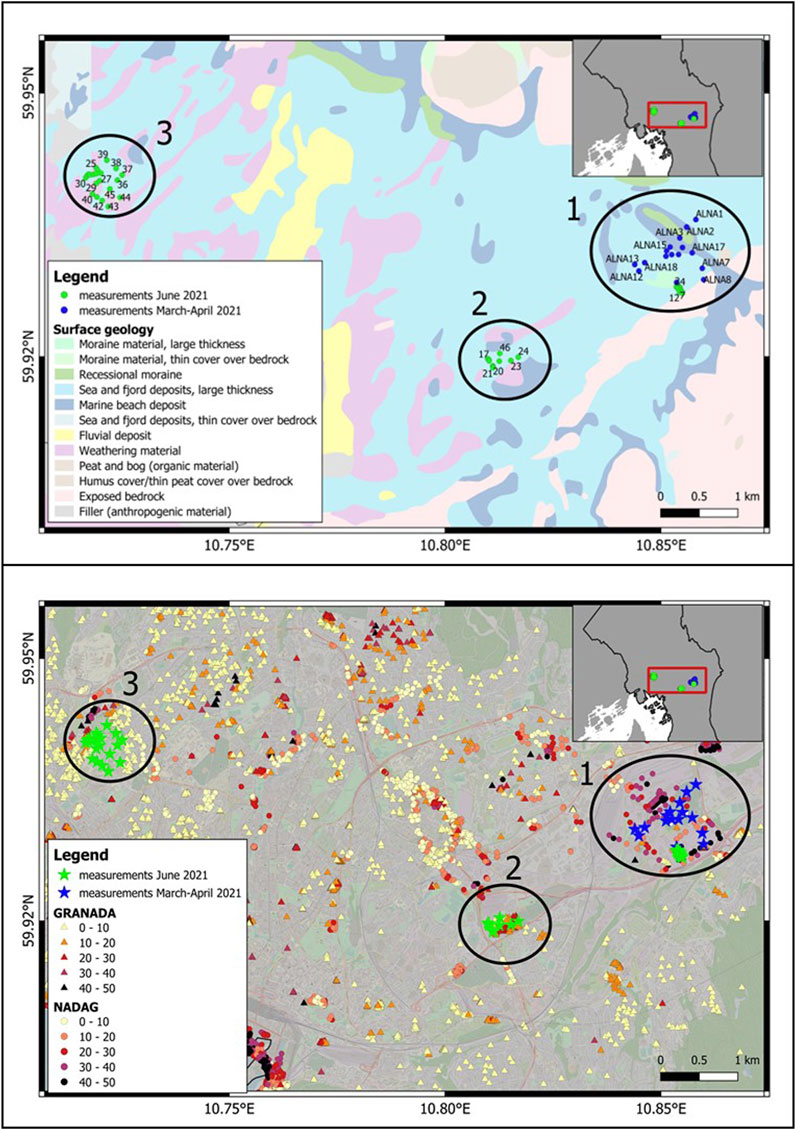
FIGURE 1. The two maps are showing fieldwork locations and HVSR measurements. In the upper right of each panel, the figure shows the municipality border of Oslo (with black line) and the red square is showing the extent of the main figure. In addition, the white area represents water, i.e., the Oslo fjord. The top panel shows a map of surface-exposed geological units together with fieldwork locations where HVSR measurements were performed (1, 2 and 3 areas). The bottom panel shows HVSR measurements together with borehole data from GRANADA (triangles) and NADAG (circles) with color-coded measured depth to basement.

3 Data and methods

We here propose an integrated approach that estimates Vs30 using the Horizontal to Vertical Spectral Ratio (HVSR) method together with a combined geology-slope approach.

3.1 Horizontal to vertical spectral ratio (HVSR) approach

The Horizontal to Vertical Spectral Ratio method is used to estimate the resonant frequency of soft sediments on top of the bedrock. The method was originally proposed by Nogoshi and Igarashi (1971), and further developed by Nakamura (1989). It consists of estimating the ratio between the Fourier amplitude spectra of the horizontal (H) and vertical (V) components of the ambient seismic noise vibrations recorded by one single seismometer (e.g., Lermo and Chavez-Garcia, 1993; Lunedei and Malischewsky, 2015; Sánchez-Sesma, 2017). Peaks in the HVSR are a result of subsurface seismic velocity contrasts (or impedance contrast), with interface depth being inverse proportional to peak frequency (see Supplementary Figure S1 in the “Supplementary Material” section). The stronger the impedance contrast between bedrock and sediments, the clearer the peak in the HVSR appears. We invert the spectral ratio for the shallow subsurface structure based on the full wavefield of body and surface waves (Diffuse Wavefield Assumption, DFA) (García-Jerez et al., 2016; Sánchez-Sesma, 2017), but it has also been inverted previously by interpreting the spectral ratio as representing the frequency-dependent Rayleigh wave ellipticity (Parolai et al., 2005).

A multitude of studies exist that used the HVSR technique to estimate site effects and/or sediment thickness (Seht and Wohlenberg, 1999; Hayles et al., 2001; Parolai et al., 2002; SESAME, 2004; Bonnefoy-Claudet et al., 2006; Rosenblad and Goetz, 2010; Chouinard and Rosset, 2012; Del Monaco et al., 2013; Yilar et al., 2017; Fat-Helbary et al., 2019; Tian et al., 2019; Putti and Satyam, 2020; Ryanto et al., 2020; Xu and Wang, 2021; Chen et al., 2023). For example, Seht and Wohlenberg (1999) applied the H/V method to estimate the basin depth in alluvial filled basin in Lower Rhine Embayment (Germany). The method was applied on parts of the basin that were only a few meters thick to other parts of the basin reaching down to as far as 1.2 km in depth. These estimated depths were compared with results from wells that drilled into the basin, and they showed that the estimates were providing similar results obtained from boreholes.

HVSR is a non-invasive and relatively simple method that can be applied quickly and easily in the field without requiring drilling or excavation. It provides a direct measurement of the fundamental resonance frequency of the site, which is related to the shear wave velocity structure and can be used to estimate Vs30, for both soft soils and rock at different depths if a velocity contrast is present in the sub-surface, which can be useful in studying soil-layering effects on seismic site response.

Site effects are commonly estimated to understand expected lateral differences in strong ground motion amplitudes caused by large earthquakes which can be substantial. The HVSR method has the advantage of being applicable to regions with lower seismic activity and longer earthquake return periods since seismic noise is used instead of earthquake records.

It is important to note that the HVSR method is sensitive to various factors, such as local geology, the thickness and the type of soil, the topography at the site, the depth and strength of the velocity contrast below the sedimentary layers, and the presence of dominant noise sources in the recorded data, which can affect the accuracy of the Vs30 estimation and the HVSR method in general. The inversion of HVSR requires certain constraints on the model space (e.g., layered models with constant velocity). Furthermore, the topography can have an effect since HVSR inversion usually does not take the 3D surface into account. Moreover, potential tilt of the layers or 3D structural effects are not included, neither are here more complex layering of several impedance contrasts, as we only focus on the most dominant interface. The method also benefits a lot from a reference site with a known Vs30 value for calibration and constraining the HVSR inversion, which may not be available in some areas. It is not suitable for sites with very low shear wave velocities, such as soft clays or alluvial deposits with large thicknesses, where the fundamental resonance frequency may be too low to be measured accurately. In addition, this method shows dependency on the size of the seismic network: with a few single point measurements, as in our study, the method does not provide information on the spatial variation of Vs30 and can only be used to estimate the average Vs30 over a small area. On the contrary, the method can provide spatial variation over a large area with a denser layout and larger number of sensors. In general, it may always be useful to supplement the HVSR method with data from other site characterization techniques, as mentioned before.

The uncertainties associated with derived Vs30 values originate from the HVSR measurements itself, as just discussed, but also from the non-uniqueness and trade-offs in the inversion of velocity-depth profiles from HVSR curves, especially when not using additional data from surface wave dispersion for example,. As already mentioned above, there are also different ways to compute and invert the HVSR (Bahavar et al., 2020). The DFA method explains HVSR based on Green’s functions including the contribution of Rayleigh, Love and body waves. For this reason, the spectra of each wavefield component must be averaged separately, i.e., HVSR corresponds to a ratio of average spectra. In the traditional approach, used by the Geopsy software package (Wathelet et al., 2020), HVSR are estimated as the average of ratios (see Bahavar et al. (2020) for more details), and Geopsy includes an inversion method expecting Rayleigh wave ellipticities as input. Here, we first compute HVSR with Geopsy (well-established code) and invert them using HVInv (more realistic noise composition). We discuss and justify our choice of methods in the discussion later.

3.1.1 HVSR measurements and processing

As mentioned in the introduction, we applied the HVSR method in different parts of the Oslo area (see Figure 1). The ambient noise measurements were performed during a number of campaigns conducted in 2021. At each one of the total 61 sites, we recorded for 1 hour using a Raspberry Shake 3D seismic sensor (Figure 2).

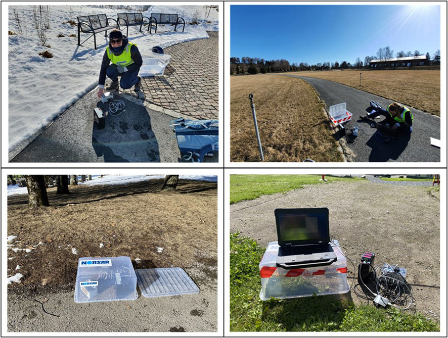
FIGURE 2. Pictures taken during fieldwork in the Alna and Blindern regions (1 and 3 area in Figure 1) in March and June 2021. On the top left, deploying the instruments at the site. On the top right, writing down the starting time of the recording and coordinates information related to the site. In the bottom left, the instrumentation is recording at the site for 1 hour. In the bottom right, downloading the recordings on the laptop.

We apply the HVSR method using Geopsy where the computation of the H/V ratio follows different steps (see Supplementary Figure S1 in the “Supplementary Material” section).

1. Start with a record of 3-component ambient noise data.

2. Divide the record in short overlapping time windows.

3. Select the most stationary time windows in order to avoid transient noise (anti-triggering algorithm).

4. Compute and smooth the Fourier amplitude spectra for each time window for each component (Z, N-S, E-W).

5. Calculate average of the two-horizontal components using a quadratic mean.

6. Compute the H/V ratio for each window.

7. Finally compute the average H/V ratio for all time windows.

We tested different parameter settings in Geopsy. The final setting was found to be optimal after qualitatively evaluating the resulting HVSR curves. The Raspberry Shake sensor has a sampling frequency of 100 Hz, so the waveforms are filtered at an upper frequency of 50 Hz. Apart from that no pre-filtering is applied before computing the waveform spectra. No overlap between time windows was used. All processing parameters are summarized in Table 1 and the results are displayed graphically with several HVSR curves.

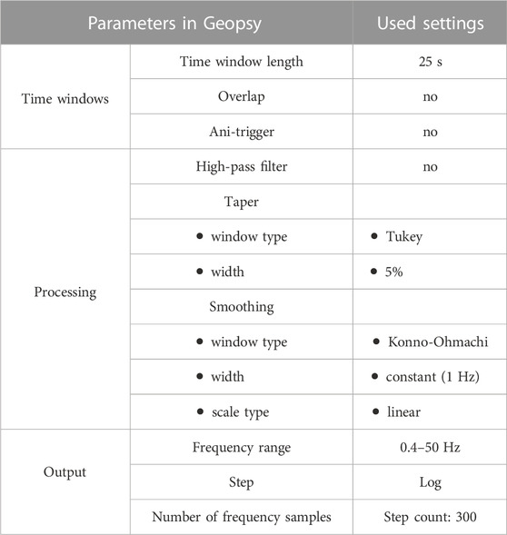
TABLE 1. List of the most relevant parameters used in Geopsy (time, processing and output) and the corresponding settings used in our study.

In Figure 3, two examples of H/V curves are shown:

1. On the left, the frequency peak with an H/V amplitude ratio equal to 4.6 is observed at relative low frequency (1.3 Hz), suggesting that the sediment cover is relatively thick. This site corresponds to site 9 and at the same location GRANADA database reports that the bedrock is at 19 m depth.

2. On the right, the frequency peak with an H/V amplitude ratio equal to 6.3 is observed at a higher frequency (29.4 Hz) and this represents thinner sedimentary cover. The H/V curve is representative of site 39. The closest GRANADA borehole is located at 67 m distance from this site and indicates that the bedrock is shallow (between 1 and 3 m depth).

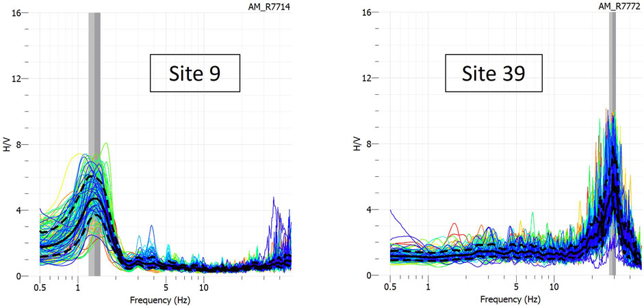
FIGURE 3. H/V plots for two different sites. On the left, site 9 shows a frequency peak at lower frequency indicative of relatively thick sediment cover on top of the bedrock. On the right, site 39 shows a frequency peak is at higher frequency indicative of a shallow cover-bedrock contact. The colored curves correspond to individual time windows. The average HVSR is shown as black curves with standard deviation (dashed).

These examples show a general agreement between the HVSR and boreholes information.

3.1.2 H/V inversion

Our measured H/V curves are used as input data for the HVInv software (García-Jerez et al., 2016) to invert for Vs depth profiles. HVInv iteratively tries to fit the H/V curves (we use 100 iterations). An example is shown in Figure 4 where the misfit for each iteration is shown. In general, the minimum frequency of the HVSRs used is 0.5 Hz and the maximum is 15 Hz (default output range of Geopsy). At certain locations with thin sediment cover we set the upper limit of the HVSR used for inversion to the Nyquist frequency of the data (50 Hz) since the maximum peak was recorded above 15 Hz.

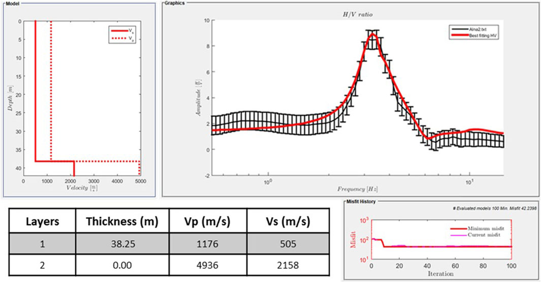
FIGURE 4. Results after using HVInv software. On the top, Vp and Vs profiles and the best H/V fit are presented. At the bottom left, the best 2-layer model and the corresponding parameters are shown. On the bottom right side misfit history is presented and shows 100 iterations.

We performed different tests to understand the sensitivity of the inverted models to the model parameter ranges. We finally decided to use the simplest model that can still explain our data reasonably well, which was in our case a single horizontal layer over a homogeneous half space, adjustable for each site where we assume homogeneous soft sediments overlying the bedrock. To avoid trade-offs between thickness and velocity, the thickness of the first layer can be fixed, for example, if prior information from borehole data is available close to the sites. The Vs. ranges are set given prior information on typical values for sediment and bedrock (NS-EN, 1998-1:2004+A1:2013+NA:2021, 2021).

- Vs min is 160 m/s and Vs max is 800 m/s for the first layer.

- Vs min is 800 m/s and Vs max is 3,400 m/s for the second layer (bedrock).

Vp ranges are set between 400 and 6,000 m/s and density between 1,500 and 3,500 kg/m³ for both layers. The algorithm inverts simultaneously for Vs, Vp and density, though HVSRs are most sensitive to Vs which is the target variable for site effect studies.

As this is likely a non-linear process, the existing algorithms could fall in local minima. Hence, we prefer a manual interaction mode, where we adjust the parameters until we are comfortable with the final mismatch, based on visual inspection. For example, in the case we do not obtain a good fit during the first inversion run, min and max Vs velocities are adjusted and secondly the thickness range of the first layer is adjusted until we obtain a good fit. Finally, we extract the best fitting model and compute the value of Vs30.

An example of the inversion procedure is given in Figure 4 (site ALNA 2). At this location, the NADAG database indicates bedrock at 38.25 m depth. We use this information to fix the thickness of the first layer. As output, the best model, fitting well the observed HVSR, gives a Vs equal to 505 m/s for the sediment layer.

After obtaining the Vs profile, the value of Vs30 is computed following the formula:

where the numerator represents the depth of 30 m and the denominator is the summation of the ratio of thickness (H_i) in meters to V_si in m/s of individual layer i within the depth of 30 m (Borcherdt, 1994; Finn and Wightman, 2004). In this case, since our first layer is thicker than 30 m, the value of Vs30 is represented only by the velocity of the layer itself.

3.2 Geology-slope approach

Wald and Allen (2007) developed a proxy-based method based on a hybrid geology-slope approach for Vs30 estimations, originally intended for inaccessible and large-scale regions where no in situ measurements for Vs30 have been available or these could not be conducted. They introduced an analysis based on the general concept that the near-surface soil or rock composition correlates to a certain degree with topographic slope. The assumption is that steeper topography tends to have little unconsolidated soil, such that steep slopes indicate stronger materials, hence higher Vs. Whereas in average, and in correlation with the local geology, at basins typically represent accumulations of sedimentary rocks and soil, which is characteristic for lower shear-wave velocities. This methodology was further refined for tectonically stable regions and values of Vs30 have been linked to ranges in topographic slope (Forte et al., 2019).

In general, the topographic slope represents the rate of change in elevation for each point compared with its immediate surrounding. In our approach, the topographic slope attributes are extracted from Digital Elevation Model and integrated with geological information from surface geological maps (https://geo.ngu.no/kart/losmasse_mobil/). We computed slope attribute from DEM10 (10 m horizontal-scale resolution Digital Elevation Model provided by the Norwegian Mapping Authority agency) using a Geographical Information Systems (GIS) platform (Figure 5).

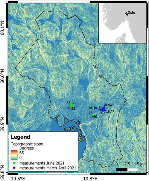
FIGURE 5. Topographic slope in degrees for Oslo area. In the figure, the border of Oslo municipality is drawn with black line and the measurement locations are shown with blue and green dots, recorded in March–April and June 2021 respectively.

Basing our approach on Forte et al. (2019), here we present for the Norwegian settings few macro classes for different surface lithology geology classes and propose Vs30 values for each macro class (Figure 6):

• Class A represents the bedrock, and the proposed value of Vs30 is >1,200 m/s.

• Class B includes thin and thick moraines sediments, and the Vs30 values range between 760 and 1,200 m/s.

• Class C is represented by fluvial sediments and the Vs30 values are 360–760 m/s.

• Class D includes marine, glacial and peat sediments with Vs.30 values between 180 and 360 m/s.

• In addition to the previous ones, class QC is added, and it represents presence of quick clay in specific areas. In this case, the value of Vs30 is fixed to 100 m/s.

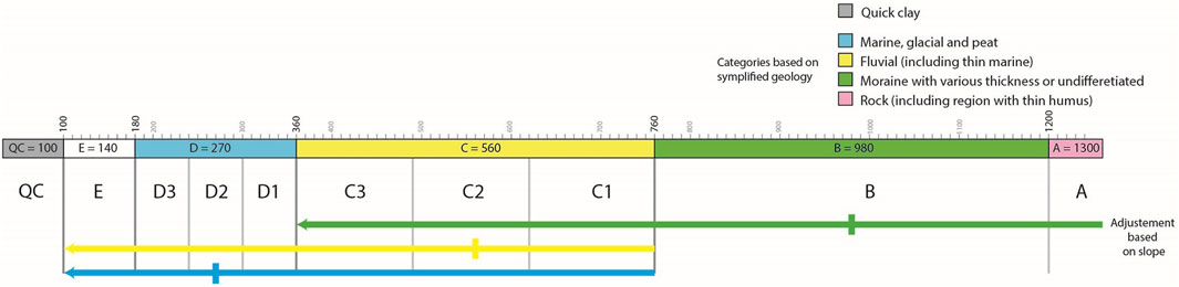
FIGURE 6. Norwegian macro classes classification of surface geology classes based on lithologies. Vs30 ranges are proposed, and adjustements based on slope values (see Table 2) can be applied for each macro class.

The slope values were then extracted on a dense grid (200 m × 200 m) and for the same grid we computed the updated values of Vs30 allowing for each macro class to vary their ranges according to slope values. Seven main ranges of slope values expressed in m/m (0.0001, 0.0045, 0.0085, 0.013, 0.022, 0.03, and 0.04) have been considered to allow the geological macro classes to be reorganized in subclasses, that can be seen in Figure 6 and in Table 2. The slope ranges (representing the ration of vertical and horizontal lengths) are taken from Wald and Allen (2007) for stable continental tectonic settings. The ranges are calibrated for DEM with a resolution of 9 arcseconds, approximately equivalent to 270 m. Consequently, to ensure compatibility with the previously mentioned calibration, a grid size of 200 m is employed for the Oslo region to extract the relevant slope value. Only using the classification based on slope values, a new class E is added allowing classes C and D to reach lower Vs30 values (class E goes from 100 to 180 m/s). The assumption regarding the utilization of slope values is correlated with the variations in the thicknesses of the sediments. Consequently, specific ranges were carefully selected to differentiate between regions where the same macro-lithologies classes were encountered, but with notable discrepancies in their respective thicknesses.

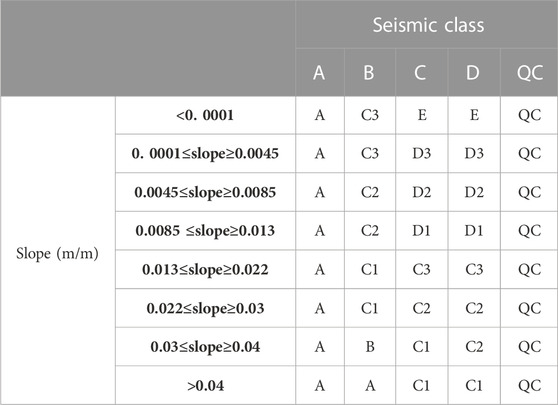
TABLE 2. New classification based on slope values (in m/m) for each macro class.

One advantage of using topographic slope to compute Vs30 is that it can provide a rough estimate of the subsurface characteristics without the need for expensive and time-consuming field measurements. The relationship between topographic slope and Vs30 is based on the fact that the slope of the land surface can influence the depth of the soil layers and the rock structure beneath it. However, calibration to the regional geology, rock types and e.g., local weathering conditions is necessary to derive more reliable correlations between Vs30 and topographic slope. Another advantage of using topographic slope to compute Vs30 is that it can be easily calculated using Digital Elevation Models and other remote sensing techniques, obtaining results for a wide area.

Understanding the topographic patterns, the main geological features and the sedimentation history provide us with qualitative information on the physical properties of the near surface (represented i.e., by Vs30). The accuracy of the derived Vs30 maps is of importance for the reliability of seismic risk calculations. Using proxies instead of acquired real data is always a simplification. However, it is important to note that topographic slope can only provide a rough estimate of Vs30, and other factors such as soil type and water content can also have a significant impact on shear wave velocities. Therefore, topographic slope should be used in connection with other methods and data sources to obtain a more accurate estimate of Vs30. This method is good at regional/national scale for seismic hazard assessment and engineering studies where no other data is available, but not at local scale; for this reason, it was used just as first evaluation and as basis to calibrate the inversion of the HVSR results (see Section 3.3).

3.3 Combined approach

We propose a combined approach that takes into account both methods explained in the previous sections. The workflow is shown in Figure 7:

1. Compute HVSR curves.

2. Perform HVSR inversion for the four pre-defined macro classes A, B, C and D. We use a one layer over half space model with the following constraining parameters:

i. The layer thickness can vary from 0 to 70 m and the Vs. ranges are defined through the macro classes (A between 1,200 and 3,400 m/s; B between 760 and 12000 m/s; C between 360 and 760 m/s and finally D between 180 and 360 m/s).

ii. The half space represents the bedrock (same as class A), and the min and max Vs. values are fixed to 1,200 and 3,400 m/s.

3. At each site we select the best fitting model and compare Vs30 of the corresponding macro class with the computed Vs30 from the geology-slope approach. To proceed, these two methods need to agree, and we accept the results of the Vs and the depth to basement. If the deviation is too large, we still perform step 4 but we assign high uncertainty to this value and encourage further measurements and quality control steps to lower that uncertainty value again.

4. We then compute the value of Vs30 at each single site based on the depth to basement and the best fitting Vs of the top layer and the basement layer and assign based on that Vs30 value a final class to the site.

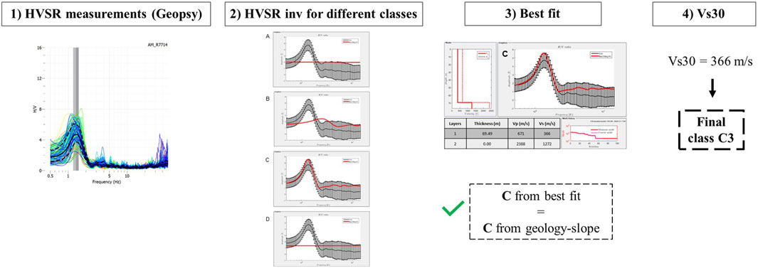
FIGURE 7. Workflow used in the combined approach. Step 1, compute HVSR curves in Geopsy. Step 2, perform HVSR inversion for the four different macro classes (A–D). One layer over half space model is used. Step 3, select the macro class that gives the best fit. Check if the macro class from the best fit corresponds to the class from the geology-slope approach. If not, we still perform step 4, but the results are treated with additional uncertainty, and we encourage further measurements and quality control steps to lower the uncertainty value. Step 4, compute Vs30 and depth to basement values from the best fit model.

As anticipated, this method does not always match the results from the previous two methods, which is a desired outcome to better identify sites with uncertain Vs30. One consideration to mention is that we are not depending on borehole information as we are not fixing the thickness of the first layer to a single value. The advantage to do that is that we get an independent estimate, where the model finds the best thickness layer to match the data. In some sites, the best fit shows a thickness of the first layer that matches the borehole’s data. Running the inversion without a fixed first layer depth makes it less constrained to derive velocity values, However, HVSR inversion without any constraints in the model space does often not perform well because of the already mentioned trade-off between depth and velocity. Hence, we have instead introduced the four macro classes, which define the boundaries for the inversion, and in addition conduct the comparison of the inversion results for the top layer and the geology-slope approach for quality control. The main advantage is that this method can be conducted without need for expensive drilling and provides results for a wider area. Moreover, borehole data are generally biased towards shallower depths, since simpler drilling techniques can stop at some hard layer or larger bolder before the actual basement is reached, and still report it as basement depth, or shallow wells never reached the basement, though final depth is falsely reported as basement. This bias becomes more pronounced for deeper sections.

4 Results

The results are presented for the three different methods, showing and comparing the estimation of the Vs30 values. For the combined approach, depth to basement estimates are also presented.

4.1 H/V curves

The H/V curves show a consistent pattern in agreement with boreholes information provided by GRANADA and NADAG databases. For example, in box 1b on the right top corner of Figure 8, we can observe that, in general, all the measurement points from 1 to 14 in Alna region are showing low frequency peak. In accordance with this observation, borehole information shows that the depth to basement in this area reaches up to 40 m depth. On the contrary, in box 3 on the right bottom corner, H/V plots are showing higher frequency peaks for Blindern area and borehole data are showing thinner sedimentary cover of only few meters.

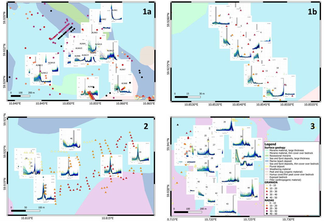
FIGURE 8. HVSR curves for the different areas (1, 2 and 3 shown in Figure 1). As background information, surface-exposed geological units and borehole data from GRANADA (triangles) and NADAG (circles) with color-coded measured depth to basement. The investigated areas show a predominant presence of sea and marine beach deposits, with local presence of moraine material in area. Panel numbers 1a, 1b, 2 and 3 are referring to the investigated areas shown in Figure 1 and Table 3.

4.2 Vs30 estimates using geology-slope approach

This method is particularly useful to provide Vs30 estimates at municipality/regional and national levels. Figure 9 shows the value of Vs30 in m/s for Oslo for a grid of 200 × 200 m. The different colors represent the different Norwegian classes presented in Figure 6. As we can observe, most of the areas outside the city center show Vs30 values for bedrock conditions. On the contrary, the area with the highest populated density is mainly represented by macro class C, represented by Vs30 values between 360 and 760 m/s. In addition, the grid results are interpolated for the entire city, using the Inverse Distance Weighting (IDW) method in GIS, and we extract Vs30 values for the measurements sites in area 1, 2 and 3. Those results are used as intermediate quality check for the combined approach. (see Figure 7).

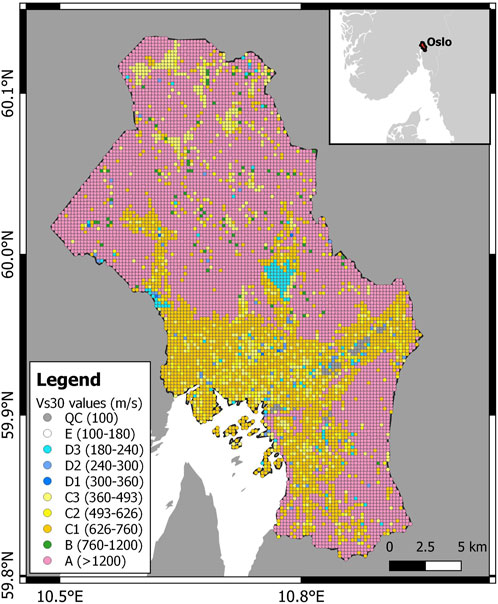
FIGURE 9. Vs30 values in m/s for the city of Oslo, obtained using the geology-slope approach. The results are displayed for 200 m × 200 m grid. The different classes are using the same color scale shown in Figure 6. The area of the city center is represented by macro class C. On the contrary, the area in the forest by macro class A since the bedrock is exposed to the surface.

4.3 Vs30 and depth to basement estimates using combined approach

The workflow presented in Section 3.3 is applied to all 61 sites and in Table 3 a summary of Vs30 and depth to basement values are shown.

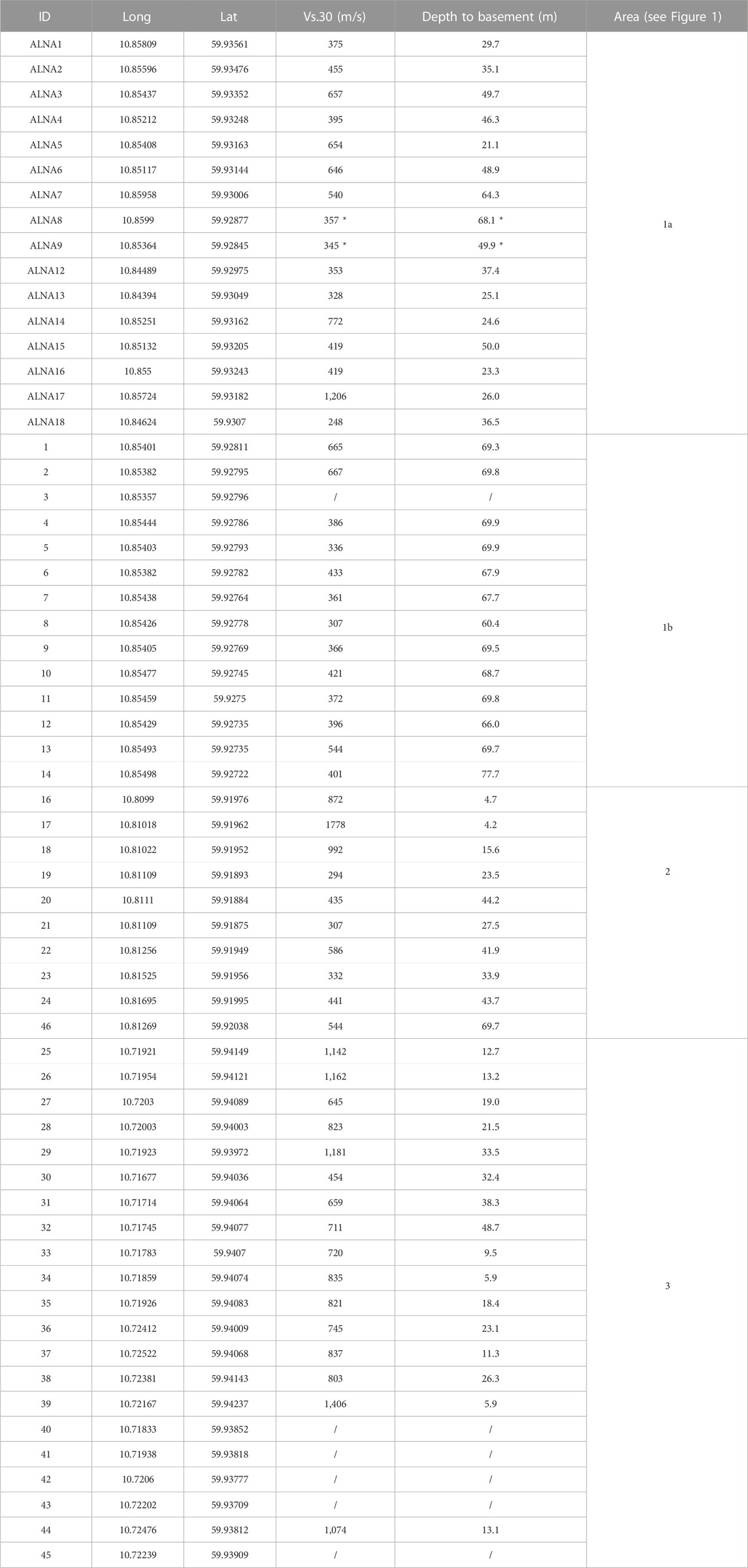
TABLE 3. Results for all 61 sites using the combined approach. The table provides the id name of the site, longitude and latitude, Vs30 (in m/s) and depth to basement (in m), and the area where each site is included (see Figure 1). The symbol “/” indicates a lack in resulting data for the Vs30 and depth to basement for sites 3, 40, 41, 42, 43 and 45 because we could not obtain a good fit with the model. Values marked with * have associated high uncertainties (due to deviations in methods) and should be treated with extra care until additional investigations may confirm the actual values.

Table 3 displays the geographic coordinates, Vs30 and depth to basement for a set of locations in Oslo. The Vs30 values range from 248 m/s to 1778 m/s indicating variations in the underlying geology and soil characteristics of the locations. The depth to basement values range about 4 m–80 m, which reflects the depth of the bedrock or competent rock beneath the soil. In some cases, we could not obtain a good fit, with the simplified model, which is then expressed by a lack in resulting data for the Vs30 and depth to basement (sites 3, 40, 41, 42, 43 and 45) (see Table 3).

Considering the location of the measurements (see Figure 1), we can observe a clear trend of lower Vs30 values and deeper depth to basement in the coastal areas compared to the inland regions, which can be attributed to glacial and marine deposits in the coastal areas. The marine boundary is defined as the highest level the sea reached after the last ice age. The boundary in Oslo lies at elevations of between approx. +200 and +210 m above sea level. Up to this level, quick clay can potentially be found. The main reason for taking the marine boundary into account is to investigate whether there is quick clay in areas where development is planned, since overloaded quick clay can lead to quick clay landslides.

4.3.1 Validation using COHIBA tool for Alna case study

In order to check the validity of the depth to basement measurements, we compare the values to borehole information nearby. This comparison is done by creating elevation maps of the top of the basement, where the difference between topography and the basement elevation gives the thickness of the sediment layer. The maps are created using a surface mapping tool called COHIBA (Abrahamsen et al., 2022; Vázquez et al., 2022). COHIBA is well suited for bringing in data from different sources such as wells, seismic interpretations, velocity models and thickness maps and producing consistent 3D maps of subsurface layers. The key to balance the relative importance of input data is to set uncertainties according to the accuracy of the data sources. COHIBA was originally developed for defining the geological structure of reservoirs offshore, but it can be applied to generate any subsurface layering, such as the near-surface basement structure.

To compare the measurements from our study to well data, we create depth to basement maps with and without our measurements and investigate the difference. This allow us to look at differences in thicknesses also when there are no obvious well-measurement pair to compare directly. To establish the depth to basement map from wells, we use COHIBA to combine the well data information. The process is as follows:

1. Define the modelled layers, which in this case is topography (taken from DEM10) and the basement.

2. Let the well data (taken from the NADAG and GRANADA databases) predict the geometry and depth of the basement structure.

3. The difference between the topography and basement will give depth to basement map for the region.

COHIBA requires a few model parameters to be set, such as well influence range on the geometry. We select a variogram ellipsoid with long axis range of 500 m, and orthogonal short axis of 300 m, with an anisotropy of 60° following the main trench structure under Alna. The well data is obtained from different drilling techniques, and the reliability and quality of the well data is rather variable, though not well documented. To acknowledge that the dataset may not be exact, we set a well data uncertainty of 0.5 m, which means that the basement surface will try to match the well data within 1–1.5 m (2-3 standard deviations) if exact conditioning is not possible. Moreover, in the case of inconsistent well data depths, COHIBA will select the best fit given data either by rejecting outliers or adding uncertainties to the well data automatically. Figure 10A shows the resulting basement structure color coded with depth to basement for a region around the Alna samples.

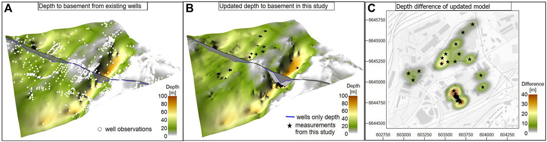
FIGURE 10. (A) Map of the basement around the Alna area (Oslo) seen from the south-west using well data from the NADAG and GRANADA databases shown as white circles. (B) Basement map updated with measurements from this study shown as black stars. (C) Difference between the two maps shown in a plan map-view, where larger values means that the updated map has a deeper basement.

To create a map using our measurements, we use the depth to basement model created by wells as input, and let our interpreted depths update the result. Again, COHIBA requires us to set the influence range of the measurements, and we choose a range of 150 m × 100 m with 60° azimuth. We choose relatively low values to isolate the difference around the measurements. We offset the uncertainty (standard deviation) of our data to be 2 m to account for the intrinsic uncertainty of the measuring method. Figure 10B shows the resulting basement structure map after it has been updated with the measurements from this study.

It can be difficult to distinguish the impact of our measurements by looking at the map alone, so the difference between the wells-only and updated map is shown in Figure 10C, where larger values mean that the measurements create a deeper map compared to the well-based map. As can be seen, since all difference values are positive, our measurements predict consistently deeper basement than the wells. The differences are in the order of magnitude of 10–20 m, with a few outliers up to 40 m deeper. This effect tends to be more pronounced for the deeper measurements than the shallow, and larger on the edges of the main trench than in the center of deeper regions.

4.4 Comparison of the three methods for some example sites

Figure 11 presents the comparison between the three methods for the sites located in area 1. As we can observe, in general the HVSR approach shows the lowest Vs30 values. The geology-slope method provides smoother values, as expected from the method and the applied 200 m gridding of the slope (see measurements 1–14), and the highest Vs30 estimates compared to the other methods. Regarding the combined approach, the Vs30 estimates are in the middle between the other two methods (with the exception of few cases), and they better integrate local heterogeneities into the smoother background from the geology-slope estimates.

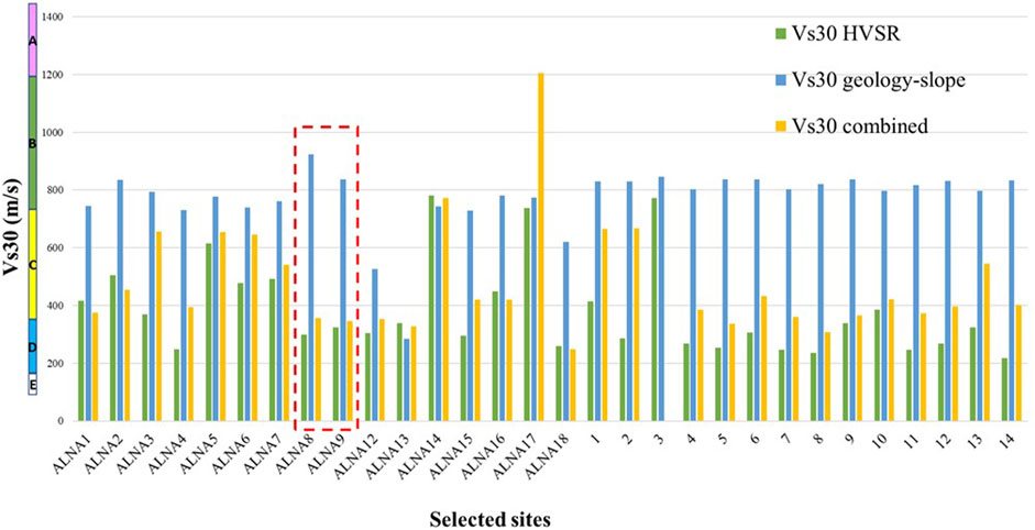
FIGURE 11. Comparison between HVSR (in green), geology-slope (in blue) and combined (in yellow) approaches to estimate Vs30 values (in m/s) in area 1. Sites ALNA 8 and ALNA 9 obtained different macro class (D1 from combined and B from geology-slope) and are hence marked with red dashed rectangle as being more uncertain.

For ALNA1, using the observations from the HVSR with constraints on the depth of the top layer (obtained in this case from nearby existing borehole data), we derive 416 m/s for the Vs30. With the geology-slope approach, we consider the exposed surface geology and combine it with the slope values, and obtain Vs30 equal to 744 m/s. The combine approach conducts the HVSR inversion for four different ranges of velocities, without fixing depths, and includes a quality check about the top layer being similar to the surface exposed geology. This is the case for ALNA1, but due to the derived thickness of almost 30 m at ALNA1, only the surface layer velocity is contributing to the Vs30, and we hence obtain a lower value of 375 m/s.

A different pattern is shown for ALNA17. The geology-slope and HVSR approaches provide very similar results, however, the combined approach indicates a higher Vs30 value. We start computing the Vs30 only through HVSR, where an inversion is conducted for one layer over half space, with some restrictions on layer thicknesses (if known from nearby well locations) and min/max Vs. The resulting best fit was estimating the Vs30 value equal to 737 m/s for the HVSR, including a depth to basement of 9 m. In the geology-slope approach, we start with the local geology that is present at the surface, regardless of the thickness of the top layer. The estimated slope value at the site allows us to update the Vs30 value and to obtain 774 m/s for the exact position of ALNA17, which is an interpolated value between the closest grid points on which Vs30 was formally computed (200 m grid). As input for the combine approach, we now used the procedure as explained in Section 3.3, with the four different macro classes defining the velocity within which HVSR inversion will be computed. The best fit was here achieved with the same macro class B as was selected from the geology-slope approach. However, the thickness of that layer was only estimated to be 26 m, and hence the resulting Vs30 (with a high basement velocity below) resulted in an estimate of 1,206 m/s. In addition, the quality control checks whether the top layer macro classification is similar, like in this case. For this reason, we have trust more the result obtained from the combined approach.

A different example is represented by ALNA8 and ALNA9, where we obtain different macro classes for the surface layer. The geology-slope approach suggests a class B for both sites, whereas the HVSR and combined approach suggest class D with a thick sedimentary layer with low velocities. In this case we still derive the Vs30 for the combined approach, but we mark the results with higher uncertainty due to the large discrepancy in the classes. In addition, we recommend a local quality check for the sites. The sites are located close to a lithological boundary, which could be a reason for the different class classification using the geology-slope approach. However, also the HVSR data could be affected from structural effects. Denser measurements could be performed in the area to reduce the uncertainty for the region.

5 Discussion

Regarding the HVSR method, there are different ways to compute HVSR which may potentially have an effect on the results. In order to evaluate the stability of the HVSR curves we adapted the code of Bahavar et al. (2020) and computed HVSR as suggested for the DFA method and compare it with the traditional method, our primary HVSR curves that we obtained using the Geopsy software. A qualitative comparison showed very similar curves, i.e., the position of the peak frequency remained stable, while some variations of amplitudes occurred (see Figure 12). The main differences are observed at frequencies lower than 1 Hz. These instabilities are most likely due to frequencies too far below the natural frequency of our sensor (4.5 Hz) and which are sensitive to deeper structures. Since the amplitude response (decay below natural frequency) of vertical and horizontal components of the sensor are the same, the spectral ratio should in theory still produce the correct site HVSR, given that instrumental noise does not dominate the data. Prior to the measurements, we performed huddle tests with co-located Raspberry Shakes sensors and short-period/broadband seismometers and found that the instrumental self-noise becomes larger than the recorded ground motion below 0.1 Hz (see Supplementary Figure S2 in the “Supplementary Material” section). Since we focus on the shallow sub-surface, the impact will therefore not be significant. In fact, the HVSR from the Raspberry Shakes and a co-located short-period seismometer at one of the instrument test sites, showing a HVSR peak at 2 Hz, looked almost identical (see Supplementary Figure S3 in the “Supplementary Material” section). However, at sites with deeper velocity contrasts, higher quality instruments with lower natural frequencies are still recommended to be used.

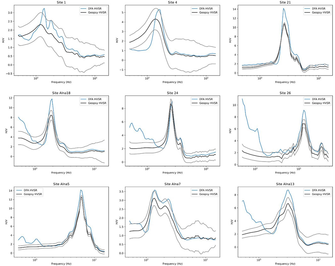
FIGURE 12. Comparison of HVSR for selected sites computed with Geopsy (mean and standard deviation of HVSR for each time window) and the DFA method (HVSR of averaged component spectra).

We run HVSR inversion for all sites again using the curves obtained with the DFA method. We do not obtain any clear trend towards decreased or increased Vs30 or basement depth. For most sites, the variation is below 20% which reflects the general uncertainty of HVSR inversion. However, for a few sites (sites ALNA1, ALNA2, ALNA3, ALNA16, 19, 46, 32, 33) slightly larger changes in the inverted models are obtained which shows that HVSR measurements must be interpreted carefully. Overall, this additional analysis helped us to get an impression about the uncertainty associated with our results. Based on this comparison, we have decided to proceed with the HVSR curves computed with Geopsy for presenting the inversion results and further use them in the combined approach. If one wants to be 100% consistent when using HVinv for HVSR inversion, we recommend computing the HVSR exactly as required for DFA. However, since there is at this point no complete program package available (only python code for long records that has to be adapted for short-term measurements), using the established Geopsy software may be more practical for many users, and as we show, seems not to affect results significantly, at least for shallow structures as in our case.

In summary, this study confirms that the HVSR method is a useful technique for estimating Vs30, but it has its limitations and should be used in conjunction with other methods and data sources for a more accurate assessment of seismic site response.

From our experience gained in the presented work, we propose a practical, reliable and useful workflow to be applied when estimating Vs30 and depth to bedrock to a larger region, such as the entire municipality of Oslo. The first step would be to conduct HVSR measurements on a rather coarse resolution with about 500 m grid distance, for instance in a 5-by-10 km area, which would result in 200 measurement points. The next step, that should be conducted in parallel to the HSVR field campaign and the analysis of each H/V curve, would be to apply the geology-slope approach to the whole region. This map would provide a first order and spatially smooth approximation for the Vs30 of the top layer. Some other studies also investigated how the topographic slope and higher-order properties derived from the topography could be used to better characterize Vs30 and depth to basement (Oye et al., 2008; Lemoine et al., 2012). These higher order properties include e.g., catchment area, downslope-slope, slope azimuth, absolute elevation and wetness index. Ground truthing of the derived Vs30 and/or depth to basement was lacking, and these authors also discuss tradeoffs between using more parameters and transfer applicability for new/other areas. We therefore propose to start using the geology-slope approach. Finally, conducting the combined approach, integrating the geological slope approach with the HVSR, will give a good overview about the match between the methods and in which areas larger misfits would be observed. This combined approach still has the advantage of being a non-invasive method, in addition it is more reliable and provides a measure of uncertainty to the results. A remaining disadvantage is that HVSR measurements need to be conducted locally, and extrapolation is not valid. In areas where larger differences would be observed, more HVSR measurements should be conducted to better probe the subsurface there. Also, in regions of special interest, e.g., where new infrastructure is planned, denser measurements could be included in generating Vs30 and depth to basement maps. In addition, all available well data should certainly be integrated in this approach using the earlier explained COHIBA method.

To validate the method, the COHIBA tool (Abrahamsen et al., 2022) was used on the Alna case study. The results show deeper depth to basement values compared to the GRANADA and NADAG boreholes databases. There may be at least two reasons for why our data is deeper; one which could imply that the measurements using this technique tend to overestimate the depth to basement, and another which suggests that wells tend to underestimate the same depth, or a combination of factors.

One potential source of error is that both well databases contain entries that have not entered the basement rock at its final drilling depth, and as such provide only a minimum depth to basement estimate. In some other cases, boulders or obstacles have been encountered while drilling, and this could also provide a mistakenly too shallow depth to basement estimate in the well database. This well data bias only goes towards shallower basement, and the effect will naturally be stronger for deeper sections. Hence, a map using only well data could potentially underestimate the depth to basement, which could also explain part of the reason why some of our measurements are deeper.

However, since none of the measurements predicts a shallower basement than the wells, there is an indication that the method overestimates the depths by about 5–10 m in general, and that the overestimation may be higher for larger depths. However, we have still shown that the method is good at separating thin sediment covers from thick and gives an overall consistent prediction with what can be estimated from wells, and it provides significant value to fill in regions between well locations. Where the difference is as much as 40 m, we are at the edge of the deep trench, and this suggests a lateral component of uncertainty where the results are influenced by neighboring regions of sediment. Most likely the actual basement depths are something in between the well data and our measurements, and this highlights the added value of using all available information when creating detailed estimates of the underground conditions.

6 Conclusion

This work shows an alternative and efficient method to estimate Vs30 values and depth to basement data. The Vs30 value is the most important attribute to characterize the soil type and subsequently account for soil type related seismic amplification. Although the Vs30 parameter is a key element in seismic hazard and risk assessments, the Vs30 is not the only factor controlling ground-motion amplification. In addition to topographic effects, the effects of deep sedimentary basins can also greatly modify the level of ground shaking observed at sites located within them and thus should be considered in combination with shallow seismic site conditions. At present, a method that can automatically delineate sedimentary basins from topographic data alone has not been developed.

To further explore the combined approach and COHIBA model’s potential, future work can involve testing them in different areas of Oslo and Norway with varying soil conditions. We believe that these tools offer a powerful, non-invasive and cost-effective solution for obtaining accurate estimations of depth to basement.

In conclusion, this approach is providing valuable information for seismic hazard assessments, geotechnical investigations and engineering design, as it can help estimate the amplification of ground motions during earthquakes, which is dependent on the soil properties and depth to bedrock. Overall, this study highlights the importance of understanding the geological and geotechnical characteristics of an area in order to accurately assess the seismic hazard and potential impacts of earthquakes. Those results can be used in earthquake hazard models and support decision-making processes related to land use planning, building codes, and emergency preparedness measures in earthquake-prone regions.

Data availability statement

The raw data supporting the conclusion of this article will be made available by the authors. Some data analyzed in this study was obtained from the Oslo municipality, some restrictions apply. Requests can be made to the corresponding author.

Ethics statement

This study incorporates the General Data Protection Regulation (GDPR) approved. The study does not involve any human participants or addresses any ethical issues.

Author contributions

FG is the main author of the article. She focused on the abstract, introduction, data, results, discussion and conclusion sections. She prepared all the pictures in the article. Her main contribution to the research work is represented by fieldwork in Oslo, performing the analysis and analyzing the results. AK, as second author, assisted FG during the H/V analysis and he contributed to the methodology, results, discussion and conclusion sections. He prepared python scripts for initial analysis of the data. AD helped to develop and implement the geology-slope approach and she prepared some figures. She also contributed writing and reviewing the paper. IA worked on creating depth to basement maps (Figure 10) using the new measurements and well data. She took part in writing the results and discussion sections and reviewed the paper. VO helped the discussion with the other authors regarding the best approach to develop the research and the article itself. He contributed to the writing and review processes. All authors contributed to the article and approved the submitted version.

Funding

The results and the research showed in this article are connected to the GEObyIT project, funded by the Research Council of Norway (Grant Number. 311596).

Acknowledgments

The authors are grateful for the economic support provided by the Research Council of Norway (Project GEObyIT, no. 311596) and to Oslo commune “Vann og Avløpsetaten” and “Plan og Bygningsetaten” departments for sharing the detailed and full borehole database for Oslo. We acknowledge the use of the Roxar RMS software for creating the depth to basement figure and using the integrated version of COHIBA.

Conflict of interest

The authors declare that the research was conducted in the absence of any commercial or financial relationships that could be construed as a potential conflict of interest.

Publisher’s note

All claims expressed in this article are solely those of the authors and do not necessarily represent those of their affiliated organizations, or those of the publisher, the editors and the reviewers. Any product that may be evaluated in this article, or claim that may be made by its manufacturer, is not guaranteed or endorsed by the publisher.

Supplementary material

The Supplementary Material for this article can be found online at: https://www.frontiersin.org/articles/10.3389/feart.2023.1242679/full#supplementary-material

References

Abrahamsen, P., Dahle, P., Kvernelv, V. B., Sektnan, A., Vazquez, A. A., and Aarnes, I. (2022). COHIBA user manual version 7.1. Oslo, Norway. Available at: https://nr.no/en/industries/natural-resources/cohiba/.
Bahavar, M., Spica, Z. J., Sánchez-Sesma, F. J., Trabant, C., Zandieh, A., and Toro, G. (2020). Horizontal-to-vertical spectral ratio (HVSR) IRIS station toolbox. Seismol. Res. Lett. 91, 3539–3549. doi:10.1785/0220200047
Bonnefoy-Claudet, S., Cornou, C., Bard, P. Y., Cotton, F., Moczo, P., Kristek, J., et al. (2006). H/V ratio: A tool for site effects evaluation. Results from 1-D noise simulations. Geophys. J. Int. 167, 827–837. doi:10.1111/j.1365-246X.2006.03154.x
Borcherdt, R. D. (1970). Effects of local geology on ground motion near san francisco bay. Bull. Seismol. Soc. Am. 60, 29–61. doi:10.1785/BSSA0600010029
Borcherdt, R. D. (1994). Estimates of site-dependent response spectra for design (methodology and justification). Earthq. Spectra 10, 617–653. doi:10.1193/1.1585791
Bungum, H., and Alsaker, A. (1991). Source spectral scaling inversion for two earthquake sequences offshore Western Norway. Bull. - Seismol. Soc. Am. 81, 358–378. doi:10.1785/BSSA0810020358
Bungum, H., Olesen, O., Pascal, C., Gibbons, S., Lindholm, C., and Vestøl, O. (2010). To what extent is the present seismicity of Norway driven by post-glacial rebound? J. Geol. Soc. Lond. 167, 373–384. doi:10.1144/0016-76492009-009
Bungum, H., Pettenati, F., Schweitzer, J., Sirovich, L., and Faleide, J. I. (2009). The 23 october 1904 MS 5.4 Oslofjord earthquake: Reanalysis based on macroseismic and instrumental data. Bull. Seismol. Soc. Am. 99, 2836–2854. doi:10.1785/0120080357
Castellaro, S., Mulargia, F., and Rossi, P. L. (2008). Vs30: Proxy for seismic amplification? Seismol. Res. Lett. 79, 540–543. doi:10.1785/gssrl.79.4.540
Castellaro, S., and Mulargia, F. (2009). VS30 estimates using constrained H/V measurements. Bull. Seismol. Soc. Am. 99, 761–773. doi:10.1785/0120080179
Chen, Z., Yao, H., Shao, X., Luo, S., and Yang, H. (2023). Detailed sedimentary structure of the Mianning segment of the Anninghe fault zone revealed by H/V spectral ratio. Earthq. Res. Adv., 100232. doi:10.1016/j.eqrea.2023.100232
Chouinard, L., and Rosset, P. (2012). “On the use of single station ambient noise techniques for microzonation purposes: The case of montreal,” in Shear wave veloc. Meas. Guidel. Can. Seism. Site charact. Soil rock. Editors J. A. Hunt, and H. L. Crow (Ottawa, Ontario: Geological Survey of Canada), 85–93.
Danciu, L., Nandan, S., Reyes, C., Basili, R., Weatherill, G., Beauval, C., et al. (2021). The 2020 update of the European seismic hazard model - eshm20: Model overview. EFEHR technical report 001 v1.0.0. 1–121. Available at: https://www.earth-prints.org/bitstream/2122/15520/1/EFEHR_TR001_ESHM20.pdf.
Del Monaco, F., Tallini, M., De Rose, C., and Durante, F. (2013). HVNSR survey in historical downtown L’Aquila (central Italy): Site resonance properties vs. subsoil model. Eng. Geol. 158, 34–47. doi:10.1016/j.enggeo.2013.03.008
Fat-Helbary, R. E. S., El-Faragawy, K. O., and Hamed, A. (2019). Application of HVSR technique in the site effects estimation at the south of Marsa Alam city, Egypt. J. Afr. Earth Sci. 154, 89–100. doi:10.1016/j.jafrearsci.2019.03.015
Finn, W. D. L., and Wightman, A. (2004). Erratum: Ground motion amplification factors for the proposed 2005 edition of the National Building Code of Canada. Can. J. Civ. Eng. 31, 718–278. doi:10.1139/L04-069
Forte, G., Chioccarelli, E., De Falco, M., Cito, P., Santo, A., and Iervolino, I. (2019). Seismic soil classification of Italy based on surface geology and shear-wave velocity measurements. Soil Dyn. Earthq. Eng. 122, 79–93. doi:10.1016/j.soildyn.2019.04.002
Fredin, O., Bergstrøm, B., Eilertsen, R., Hansen, L., Longva, O., Nesje, A., et al. (2013). “Glacial landforms and Quaternary landscape development in Norway,” in Quaternary geology of Norway (Geological Survey of Norway Special Publication).
García-Jerez, A., Piña-Flores, J., Sánchez-Sesma, F. J., Luzón, F., and Perton, M. (2016). A computer code for forward calculation and inversion of the H/V spectral ratio under the diffuse field assumption. Comput. Geosci. 97, 67–78. doi:10.1016/j.cageo.2016.06.016
Ghione, F., Mæland, S., Meslem, A., and Oye, V. (2022). Building stock classification using machine learning: A case study for Oslo, Norway. Front. Earth Sci. 10, 1–11. doi:10.3389/feart.2022.886145
Hansen, R. A., Bungum, H., and Alsaker, A. (1989). Three recent larger earthquakes offshore Norway. Terra Nov. 1, 284–295. doi:10.1111/j.1365-3121.1989.tb00371.x
Hayles, K. E., Ebel, J. E., and Urzua, A. (2001). Microtremor measurements to obtain resonant frequencies and ground shaking amplification for soil sites in Boston. Civ. Eng. Pract. 16.
Jerkins, A. E., Oye, V., Alvizuri, C., Halpaap, F., Kværna, T., and Gharti, H. N. (2023). The 21 March 2022 tampen Spur Mw 5.1 earthquake, north sea: Location, moment tensor, and aftershocks. BSSA in prep.
Junek, W. N., Kværna, T., Pirli, M., Schweitzer, J., Harris, D. B., Dodge, D. A., et al. (2015). Inferring aftershock sequence properties and tectonic structure using empirical signal detectors. Pure Appl. Geophys. 172, 359–373. doi:10.1007/s00024-014-0938-0
Lemoine, A., Douglas, J., and Cotton, F. (2012). Testing the applicability of correlations between topographic slope and VS30 for Europe. Bull. Seismol. Soc. Am. 102, 2585–2599. doi:10.1785/0120110240
Lermo, J., and Chavez-Garcia, F. J. (1993). Site effect evaluation using spectral ratios with only one station. Bull. - Seismol. Soc. Am. 83, 1574–1594. doi:10.1785/bssa0830051574
Lunedei, E., and Malischewsky, P. (2015). A review and some new issues on the theory of the H/V technique for ambient vibrations. Geotech. Geol. Earthq. Eng. 39, 371–394. doi:10.1007/978-3-319-16964-4_15
Morelli, T. A. (2013). Depth to bedrock estimations using the H/V spectral ratio in the san joaquin valley. Available at: http://repositorio.uchile.cl/bitstream/handle/2250/130118/Memoria.pdf.
Nakamura, Y. (1989). Method for dynamic characteristics estimation of subsurface using microtremor on the ground surface. Q. Rep. RTRI Railw. Tech. Res. Inst. 30.
Nakamura, Y. (2008). “On the H/V spectrum,” in The 14th World Conference on Earthquake Engineering, Beijing, China, October 12-17, 2008, 1–10.
Neumann, E. R., Olsen, K. H., Baldridge, W. S., and Sundvoll, B. (1992). The Oslo Rift: A review. Tectonophysics 208, 1–18. doi:10.1016/0040-1951(92)90333-2
Nielsen, J. K., and Nielsen, J. K. (2007). Landet blir til - Norges geologi. GeologiskNyt 17 (4). doi:10.7146/gn.v0i4.3409
Nogoshi, M., and Igarashi, T. (1971). On the amplitude characteristics of microtremor (Part 2). Zisin J. Seismol. Soc. Jpn. 2nd ser.) 24, 26–40. doi:10.4294/zisin1948.24.1_26
NS-EN 1998-1:2004+A1:2013+NA:2021 (2021). Eurocode 8 — design of structures for earthquake resistance — Part 1: General rules, seismic actions and rules for buildings. Available at: https://www.phd.eng.br/wp-content/uploads/2015/02/en.1998.1.2004.pdf.
Oye, V., Bungum, H., Etzelmüller, B., and Lindholm, C. (2008). “On the use of multiple terrain parameters as a proxy for sediment thickness (depth to basement): Case study for Norway,” in Report of network of research infrastructures for European seismology (NERIES) – jra3.
Parolai, S., Bormann, P., and Milkereit, C. (2002). New relationships between Vs, thickness of sediments, and resonance frequency calculated by the H/V ratio of seismic noise for the cologne area (Germany). Bull. Seismol. Soc. Am. 92, 2521–2527. doi:10.1785/0120010248
Parolai, S., Picozzi, M., Richwalski, S. M., and Milkereit, C. (2005). Joint inversion of phase velocity dispersion and H/V ratio curves from seismic noise recordings using a genetic algorithm, considering higher modes. Geophys. Res. Lett. 32, L01303. doi:10.1029/2004GL021115
Pirli, M., Schweitzer, J., Ottemöller, L., Raeesi, M., Mjelde, R., Atakan, K., et al. (2010). Preliminary analysis of the 21 February 2008 Svalbard (Norway) seismic sequence. Seismol. Res. Lett. 81, 63–75. doi:10.1785/gssrl.81.1.63
Pirli, M., Schweitzer, J., Paulsen, B., Konechnaya, Y. V., and Antonovskaya, G. N. (2021). Two decades of seismicity in storfjorden, svalbard archipelago, from regional data. Seismol. Res. Lett. 92, 2695–2704. doi:10.1785/0220200469
Pirli, M., Schweitzer, J., and Paulsen, B. (2013). The Storfjorden, Svalbard, 2008-2012 aftershock sequence: Seismotectonics in a polar environment. Tectonophysics 601, 192–205. doi:10.1016/j.tecto.2013.05.010
Putti, S. P., and Satyam, N. (2020). Evaluation of site effects using HVSR microtremor measurements in vishakhapatnam (India). Earth Syst. Environ. 4, 439–454. doi:10.1007/s41748-020-00158-6
Ramberg, I. B., Bryhni, I., Arvid, N., and Rangnes, K. (2008). The making of a land; geology of Norway. Trondheim, Norway: Norwegian Geological Society.
Ro, H. E., and Faleide, J. I. (1992). A stretching model for the Oslo Rift. Tectonophysics 208, 19–36. doi:10.1016/0040-1951(92)90334-3
Rosenblad, B. L., and Goetz, R. (2010). Study of the H/V spectral ratio method for determining average shear wave velocities in the Mississippi embayment. Eng. Geol. 112, 13–20. doi:10.1016/j.enggeo.2010.01.006
Ryanto, T. A., Iswanto, E. R., Indrawati, Y., Setiaji, A. B., and Suntoko, H. (2020). Sediment thickness estimation in serpong experimental power reactor site using HVSR method. J. Pengemb. Energi Nukl. 22, 29. doi:10.17146/jpen.2020.22.1.5949
Sánchez-Sesma, F. J. (2017). Modeling and inversion of the microtremor H/V spectral ratio: Physical basis behind the diffuse field approach. Earth, Planets Sp. 69, 92. doi:10.1186/s40623-017-0667-6
Seht, M. I. V., and Wohlenberg, J. (1999). Microtremor measurements used to map thickness of soft sediments. Bull. Seismol. Soc. Am. 89, 250–259. doi:10.1785/bssa0890010250
SESAME (2004). “Guidelines for the implementation of the H/V spectral ratio technique on ambient vibrations-measurements, processing and interpretations, SESAME European research project,” in SESAME site eff. Assess. Using ambient excit.
Singh, S. K., Lermo, J., Dominguez, T., Ordaz, M., Espinosa, J. M., Mena, E., et al. (1988). The Mexico earthquake of september 19, 1985—a study of amplification of seismic waves in the valley of Mexico with respect to a hill zone site. Earthq. Spectra 4, 653–673. doi:10.1193/1.1585496
Tian, B., Du, Y., You, Z., and Zhang, R. (2019). Measuring the sediment thickness in urban areas using revised H/V spectral ratio method. Eng. Geol. 260, 105223. doi:10.1016/j.enggeo.2019.105223
Vázquez, A. A., Dahle, P., Abrahamsen, P., and Sektnan, A. (2022). Conditioning geological surfaces to horizontal wells. Comput. Geosci. 26, 1223–1236. doi:10.1007/s10596-022-10154-6
Wald, D. J., and Allen, T. I. (2007). Topographic slope as a proxy for seismic site conditions and amplification. Bull. Seismol. Soc. Am. 97, 1379–1395. doi:10.1785/0120060267
Wathelet, M., Chatelain, J. L., Cornou, C., Giulio, G., DiGuillier, B., Ohrnberger, M., et al. (2020). Geopsy: A user-friendly open-source tool set for ambient vibration processing. Seismol. Res. Lett. 91, 1878–1889. doi:10.1785/0220190360
Xu, R., and Wang, L. (2021). The horizontal-to-vertical spectral ratio and its applications. EURASIP J. Adv. Signal Process 2021, 75. doi:10.1186/s13634-021-00765-z
Yilar, E., Baise, L. G., and Ebel, J. E. (2017). Using H/V measurements to determine depth to bedrock and Vs30 in Boston, Massachusetts. Eng. Geol. 217, 12–22. doi:10.1016/j.enggeo.2016.12.002
Keywords: seismic hazard, site effect, Vs30, depth to bedrock, HVSR, topographic slope
Citation: Ghione F, Köhler A, Dichiarante AM, Aarnes I and Oye V (2023) Vs30 and depth to bedrock estimates from integrating HVSR measurements and geology-slope approach in the Oslo area, Norway. Front. Earth Sci. 11:1242679. doi: 10.3389/feart.2023.1242679
Received: 19 June 2023; Accepted: 21 July 2023;
Published: 09 August 2023.
Edited by:
Sergio Molina-Palacios, University of Alicante, SpainReviewed by:
Jose Delgado, Universidad de Alicante, SpainVeronica Pazzi, University of Trieste, Italy
Copyright © 2023 Ghione, Köhler, Dichiarante, Aarnes and Oye. This is an open-access article distributed under the terms of the Creative Commons Attribution License (CC BY). The use, distribution or reproduction in other forums is permitted, provided the original author(s) and the copyright owner(s) are credited and that the original publication in this journal is cited, in accordance with accepted academic practice. No use, distribution or reproduction is permitted which does not comply with these terms.
*Correspondence: Federica Ghione, federica.ghione@norsar.no